NH-LoRA

Neuromorphic Horizontal LoRA : Future-Aware Structural Expansion of Low-Rank Adapters for Rehearsal-Free Class-Incremental Learning

Hartmann Kanisius && Syauqi Nabil Tasril ✓ 30 min read (maybe) · Apr 11, 2026

Preface

Tl;dr :

We proposed new LoRA architecture called NH-LoRA as part of PEFT on Continual Learning, spesifically on image classification. We also show it's performance on Continual Learning task with final average accuracy and forgetting.

Hello ! So... this project is a part of collaboration between me (Hartmann) and Syauqi. Anyway, this new architecture was inspired by neuromorphic computing [3], DEN [5], and CL-LoRA method [2]. The problem domain itself, Class-Incremental Learning, was relatively new and rarely discussed (at least at the time I wrote this). But, we believe it could be very useful for existing models, especially when they need to be maintained over time and able to learn new knowledge, without forget the old one. That, is what we want to address.

Oh, btw, this was make as KCVanguard Final Project, part of KCV Lab Recruitment. Maybe, we'll make the Indonesian version of this (and I'll put it here). Because this is a new architecture, there will be really, really lot of equation here. We'll try to explain them in a comprehensive, structured, and (hopefully) easy-to-understand way.

Problem Statement

Image Classification

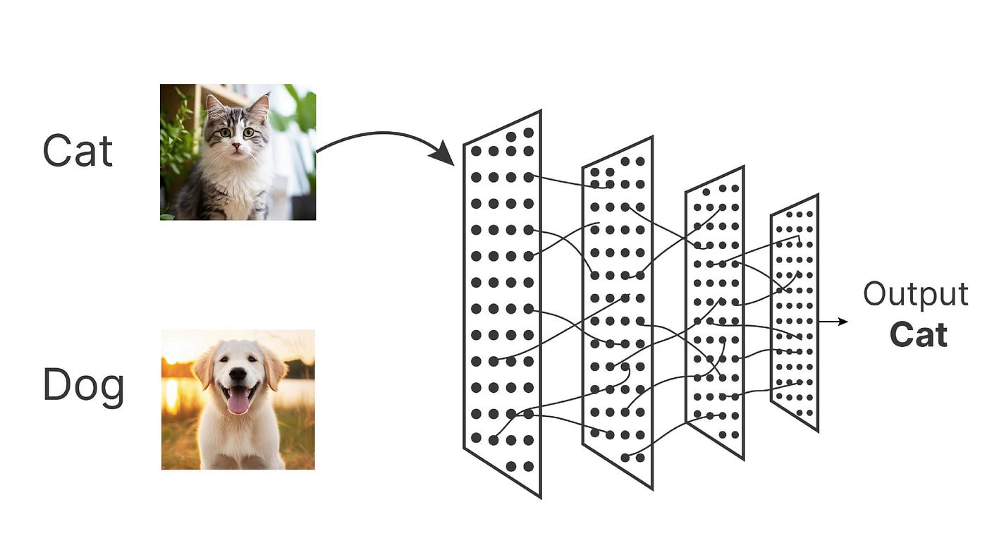
Image Classification is simply a task to give a label to an image. Every image classification model have this common idea :

Input the image
Passes it through a series of layers
Decides the most likely categories

(Incremental) Image Classification

In image classification, a model is trained on a fixed set of classes, so it only learns to recognize classes within that domain.

hmmm.... What if we want to add a new class later ?

Well, we can fine-tune or retrain the model. Let's say I chose to fine-tune because I don't have time to retraining. So the model learn the new concept well, but somehow, maybe it lose some ability to recognize the old ones at the same time. This is known as forgetting, common problems on fine-tuning.

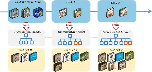
So, incremental learning can be viewed as a special task in fine-tune domain [1]. We add new classes over time while try to preserve performance on previously learned classes (Btw, we use the term incremental here, but it's similar with continual learning)

Formally, we can think of the learning process as a sequence of tasks $T_{1}, T_{2}, \dots, T_{t}$ , where each task $T_{i}$ introduces a new set of classes $C_{i}$ .

After training on task $t$ , the model should still be able to correctly classify images from all classes seen so far:

C_{total} = C_{1} \cup C_{2} \cup \dots \cup C_{t}

In short, this diagram should helps the intuition :

To deal with incremental image classification, we use vision transformer model. There are more model tho, but we use this because it's the same model that CL-LoRA use, so the benchmark can be done fairly.

Vision Transformer (ViT)

Vision Transformers (ViT) is a Transformer but for images, works by treating image patches as tokens.

Transformers? Thought that was for NLP, iirc? ... Yep, but the idea actually can be used for images as well. I think better we explained some concept here to make sure we are on the same page ....

Transformer

Transformers are models that process a sequence by letting each element compare itself with the others, instead of reading everything in a fixed (left-to-right) order [6]. Transformer is identical with attention (imo, since these two terms are often mentioned together).

... attention, like how much we put attention into something ?

Attention

I think, better if we explain these use sentence :

The animal didn't cross the street because it was too tired

In Natural Language Processing, that sentence would be converted into tokens. These can be whole words, subwords, or character pieces .. depending on the tokenizer. For this example, let's say the sentences are converted into these tokens :

The_ | animal_ | didn_ | '_ | t_ | cross_ | the_ | street_ | because_ | it_ | was_ | too_ | tire | d_

Based on the infamous paper [7], each token gets projected into three vectors, Query (Q), Key (K), Value (V), and the attention score between tokens will be :

Attention (Q, K, V) = softmax (\frac{Q K^{T}}{\sqrt{d_{k}}}) V

Now, we will use some math to find out how much it_ "pays attention" to animal_ compared to street_.

Some Math

To do so, let’s assume this hypothetical vector values that a trained model might output for these words :

Query for it_:

Q_{it} = [0.6, 0.3, - 0.4, 0.8]

Key for animal_:

K_{animal} = [0.5, 0.4, - 0.3, 0.7]

Key for street_:

K_{street} = [- 0.2, 0.1, 0.5, - 0.3]

Key for was_:

K_{was} = [0.3, 0.1, - 0.1, 0.5]

Assume $d_{k} = 4$ , so the scaling factor is:

\sqrt{d_{k}} = \sqrt{4} = 2

First, compute the raw score from it_ :

Attending to animal_:

\begin{aligned} Q_{it} \cdot K_{animal} & = (0.6) (0.5) + (0.3) (0.4) + (- 0.4) (- 0.3) + (0.8) (0.7) \\ = 0.30 + 0.12 + 0.12 + 0.56 \\ = 1.10 \end{aligned}

Attending to street_:

\begin{aligned} Q_{it} \cdot K_{street} & = (0.6) (- 0.2) + (0.3) (0.1) + (- 0.4) (0.5) + (0.8) (- 0.3) \\ = - 0.12 + 0.03 - 0.20 - 0.24 \\ = - 0.53 \end{aligned}

Attending to was_:

\begin{aligned} Q_{it} \cdot K_{was} \\ = (0.6) (0.3) + (0.3) (0.1) + (- 0.4) (- 0.1) + (0.8) (0.5) \\ = 0.18 + 0.03 + 0.04 + 0.40 \\ = 0.65 \end{aligned}

Then, we apply scaling :

[\frac{1.10}{2}, \frac{- 0.53}{2}, \frac{0.65}{2}] = [0.55, - 0.265, 0.325]

Apply softmax :

softmax ([0.55, - 0.265, 0.325]) \approx [0.45, 0.20, 0.35]

So it_ puts roughly 45% of its attention weight on animal_, 35% on was_, and 20% on street_.

The output embedding of it_ becomes a weighted blend of the value vectors, with the strongest contribution coming from animal_.

At the end, it will be something like this :

(A reminder that those are dummy numbers for visualization purposes)

(Vision) Transformer

Alright, now we know how to "count attention" with words. How those were applied to the image, to be exactly? ...

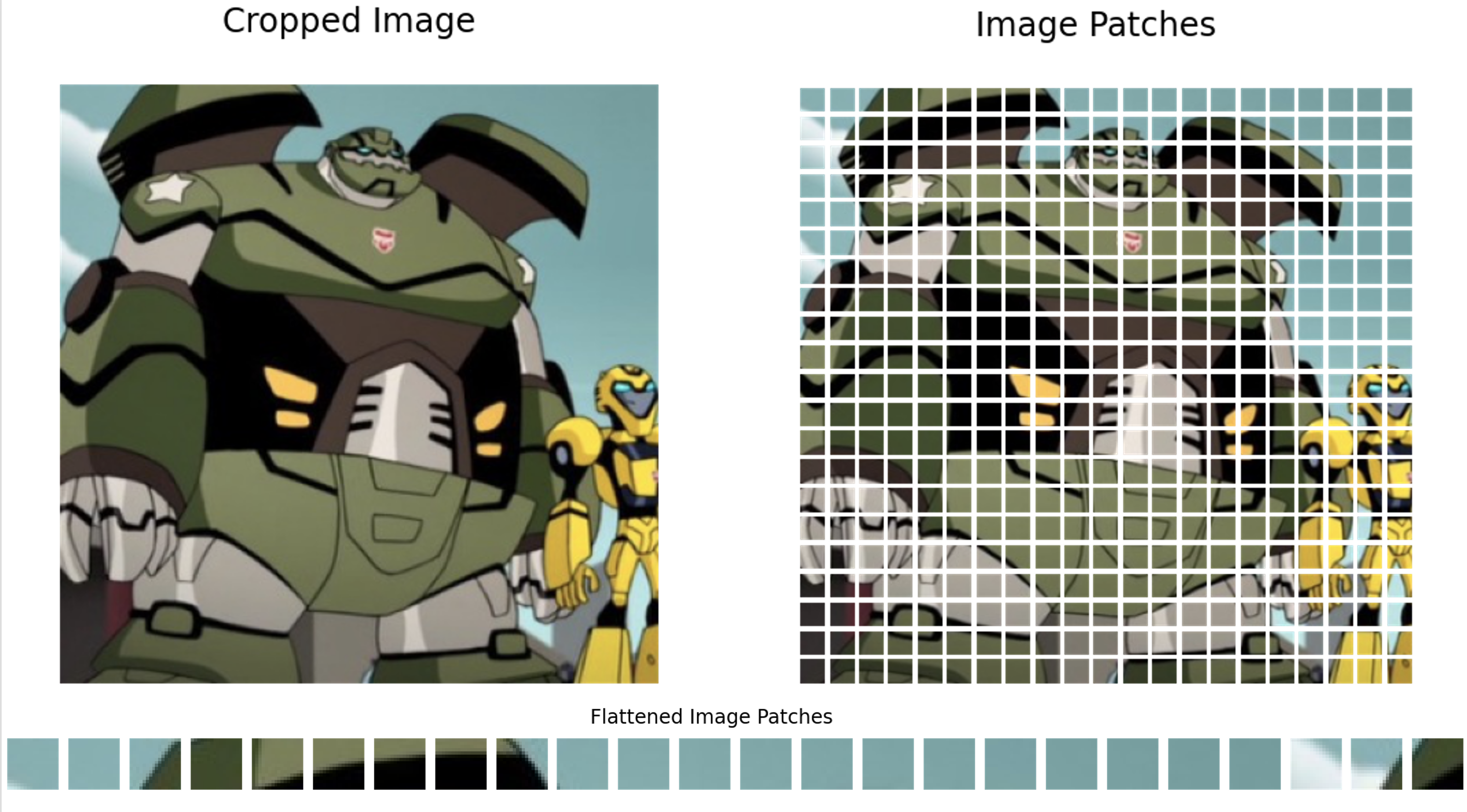
Patch Embedding

Vision Transformer works by cutting the image into patches and treating each patch like a token in a sentence. For example, a 224×224 image with patch size 16×16 :

Number of patches = \frac{224}{16} \times \frac{224}{16} = 14 \times 14 = 196 patches

Each patch is then flattened and mapped into a $D$ -dimensional embedding using a linear projection (like $[w, x, y, z]$ in attention chapter). It's called patch embedding

Positional Encoding

We have the embedding, now start count attention score ? Not really.

One problem with Transformers is we need to give the order of the input. If you shuffled all the tokens randomly and fed them... well, it still works, but it won't give good information for the model to "understand" the context. The model won't find any difference for an orange image or a scrambled orange puzzle.

With text, it's easy with text because they are ordered, like how we read them from left to right. With images... they don't have natural "reading order" the like words. Patch number 7 isn't inherently "after" patch 6 in any meaningful sense. But a patch containing something like "orange and round" can mean very different things depending on whether it appears in the top-left corner, the center, or the bottom-right. So, to solve this, we add positional embeddings

The final embedding $z_{0}$ are derived from this calculation :

z_{0} = [x_{class}; x_{p}^{1} E; x_{p}^{2} E; \dots; x_{p}^{N} E] + E_{pos}

With :

$x_{class}$ : A special, extra "classification token" prepended to the sequence (it gathers the final global image info to make a prediction).
$x_{p}^{i} E$ : This is your image patch ( $x_{p}^{i}$ ) multiplied by a linear projection matrix ( $E$ ). This just means we've squashed a patch of pixels into a vector of numbers.
$E_{pos}$ : The positional embedding matrix.

The reasoning here .. is basically to make the embedding more grouped by position.

Some Math

Let's take an example. Imagine we are looking at a picture of a landscape. Patch 1 is the top-left corner (blue sky), and Patch 16 is the bottom-right corner (which happens to be a blue lake). Visually, they might look identical.

Let's say our embedding dimension is $4$ :

Visual Embedding for Patch 1 (Sky): $[0.8, 0.2, 0.9, 0.1]$
Visual Embedding for Patch 16 (Lake): $[0.8, 0.2, 0.9, 0.1]$

If we stopped here, the model would think these two patches are the exact same thing in the exact same context. Now, let's add the positional embeddings ( $E_{pos}$ ):

Positional Embedding for Position 1 (Top-Left):
$[0.1, 0.0, 0.1, 0.0]$
Positional Embedding for Position 16 (Bottom-Right):
$[- 0.1, 0.5, - 0.1, 0.2]$

Now, we produce the final patch ( $z_{0}$ ):
Final Patch 1 Input:
$[0.8 + 0.1, 0.2 + 0, 0.9 + 0.1, 0.1 + 0] = [0.9, 0.2, 1.0, 0.1]$
Final Patch 16 Input:
$[0.8 - 0.1, 0.2 + 0.5, 0.9 - 0.1, 0.1 + 0.2] = [0.7, 0.7, 0.8, 0.3]$

Ohh? Even though the visual pixels were identical, the final embedding are different, based on the position

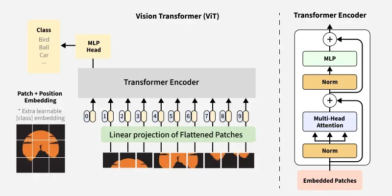
Finally, this embedding will be input for Transformer architecture, with it's attention mechanism, MLP head, yadda yadda...

In short, may this diagram helps the intuition :

NH-LoRA

Now, let's see the proposed architecture. Ehhh, wait, I think I still need to explain some terms before that.

Preface

PEFT (Parameter Efficient Tuning)

PEFT, is the "family of techniques" that fine-tune model by updating a small number of parameters. In many cases, these methods can achieve performance that is comparable to fine-tuning all model parameter. So almost same result with less time, win-win solution.

There are really lot of them (well, family technique), I think this figure should give good overview about PEFT [10].

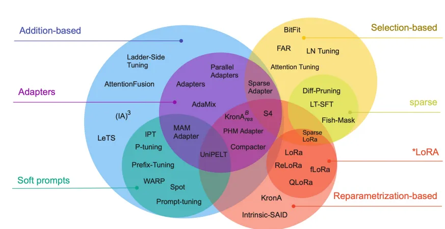
We won't explain all of them (that will be a burden), Let's just focus on LoRA.

LoRA

Okay, so LoRA stands for Low-Rank Adaption, which some technique to approximate updates on weight matrix with a "low-rank decomposition" matrix [11].

... what does that mean? Let's start with diagram for better intuiton :

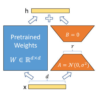
As shown in diagram, we call the original pre-trained weights as $W$ . The intuition was, during training (or fine-tuning, to be specific), we want to find a change to these weights, which we'll call $Δ W$ . Instead of learning that $Δ W$ matrix directly, we freeze the original weights $W$ and approximate $Δ W$ by multiplying two much smaller matrices together, $A$ and $B$ .

Some Math
Let's take an example. From training, "ideal" weight update $Δ W$ from a standard backprop looks like this $3 \times 3$ matrix:

Δ W = [\begin{matrix} 2 & 4 & 6 \\ 3 & 6 & 9 \\ 4 & 8 & 12 \end{matrix}]

Normally, that's $9$ separate parameters we have to update and train. But if we look closely, there's a pattern. Every row is essentially just a multiple of the sequence $[1, 2, 3]$ . Because of this redundancy (which actually happens a lot in neural networks during adaptation), we can represent this exact same matrix by taking the outer product of a $3 \times 1$ column matrix ( $A$ ) and a $1 \times 3$ row matrix ( $B$ ) at a rank size of $r = 1$ :

A = [\begin{matrix} 2 \\ 3 \\ 4 \end{matrix}]

B = [\begin{matrix} 1 & 2 & 3 \end{matrix}]

So, if we multiply $A \times B$ , we get the exact same $Δ W$ back, right ? With doing so, we only train the parameters inside $A$ and $B$ , which is $6$ parameters.

In short, We want to optimize A and B such that $A \otimes B$ is as close as possible to the actual updated $Δ W$ .

Architecture

Now, let's see the proposed architecture (this time fr).

Btw, some important terms that we'll use a lot here :

Adapter: A new module injected into each block of the network to enable parameter-efficient adaptation without modifying the original backbone weights.
Block / Layer: The terms block and layer are used interchangeably to refer to a single transformation unit in the model (e.g., a Transformer block).
Slot Representation: A slot is a latent vector (embedding) derived from the patch embeddings in a Vision Transformer (ViT), processed through an attention mechanism.

About slot, each slot serves as a compact representation of a learned subspace and is used to generate low-rank factors. Specifically, the slot is used to parameterize the LoRA matrices :

A (s) = f_{A} (s), B (s) = f_{B} (s)

where $s$ is the slot embedding, and $f_{A} (\cdot)$ and $f_{B} (\cdot)$ are learned mappings.

These factors are then used to construct the low-rank update :

Δ W (s) = B (s) A (s)

This mechanism allows each slot to dynamically control the low-rank adaptation applied to the model.

Task-State Encoder

Tasks

Remember when we talk about task in incremental image classification here ? Now.. what is a task, actually?

Task is simply a group or subset of labels. Let's say we have the full set of classes :

C = {c_{1}, c_{2}, \dots, c_{K}}

Then, these classes are divided into several task groups:

C_{1}, C_{2}, \dots, C_{T}

with the condition:

C_{i} \cap C_{j} = \emptyset for i \neq j

This means that each class belongs to only one task.

Warmup

Suppose task $t$ has the following dataset:

D_{t} = {(x_{i}, y_{i})}_{i = 1}^{n_{t}}, y_{i} \in C_{t}

Warm-up will takes a small initial batch:

B_{t} = {(x_{i}, y_{i})}_{i = 1}^{m}, m ≪ n_{t}

Let

B_{t}^{warm} = {(x_{n}, y_{n})}_{n = 1}^{N_{w}}

be the sample set from the warm-up phase.

With $f (\cdot)$ denoting the feature extractor from the frozen backbone and the currently active adapter, the task mean feature is defined as :

μ_{t} = \frac{1}{N_{w}} \sum_{n = 1}^{N_{w}} f (x_{n}) .

The feature dispersion is summarized using diagonal covariance or per-dimension variance:

σ_{t} = \frac{1}{N_{w}} \sum_{n = 1}^{N_{w}} (f (x_{n}) - μ_{t})^{⊙ 2},

where $⊙ 2$ denotes element-wise squaring.

To compute a lightweight gradient sketch over trainable parameters during warm-up, we use

g_{t} = [‖ \nabla_{Δ W_{1}} L^{warm} ‖_{2}, ‖ \nabla_{Δ W_{2}} L^{warm} ‖_{2}, \dots, ‖ \nabla_{Δ W_{M}} L^{warm} ‖_{2}],

where $L^{warm}$ is the warm-up loss and ${Δ W_{m}}_{m = 1}^{M}$ denotes the set of monitored trainable adapter modules.

To compare the current task with previous experience, a similarity signal is computed from the history bank. If

H_{t - 1} = {h_{1}, \dots, h_{t - 1}}

is the summary of previous tasks, then the similarity score is

s_{t} = {\begin{cases} 0, & t = 1, \\ max_{i \in {1, \dots, t - 1}} \cos (ψ_{s} (μ_{t}), h_{i}), & t > 1. \end{cases}

Here, $ψ_{s} (\cdot)$ is a lightweight projection so that the current mean feature lies in the same space as the historical representations.

We also measures initial uncertainty through the average prediction entropy:

e_{t} = \frac{1}{N_{w}} \sum_{n = 1}^{N_{w}} H (p_{θ} (y ∣ x_{n})),

where $H (\cdot)$ denotes Shannon entropy.

All of these statistics are then combined into a raw task vector:

h_{t} = [pool (μ_{t}); pool (σ_{t}); g_{t}; s_{t}; e_{t}] .

So, to summary this :

Input image pixels and labels $\to$ compute class centroids $(μ_{t})$ , feature dispersion $(σ_{t})$ , similarity $(s_{t})$ , entropy $(e_{t})$ , and gradient sketch $(g_{t})$ $\to$ encode all of them $\to$ History Task, as input to the Horizon Planner.

Horizon Planner

Horizon Planner receive two history :

Current History Task
Previous History Task from History Bank (if exists)

We know that Current History Task is $h_{t}$ from previous section. But how to calculate Previous History Task ?

Let's say task before current task are as follow :

H_{t - 1} = {h_{1}, h_{2}, \dots, h_{t - 1}} .

To make the planner compare the current task not only with a single past task but with the full history, NH-LoRA uses a history aggregation module conditioned on $h_{t}$ . For each new task, a query is built from the current state, while keys and values are built from all elements in the history bank:

q_{t} = W_{q} h_{t}, k_{i} = W_{k} h_{i}, v_{i} = W_{v} h_{i},

where $W_{q}$ , $W_{k}$ , and $W_{v}$ are learned projections.

The attention weight for each historical task is computed as

a_{i}^{(t)} = \frac{\exp (\frac{q_{t}^{⊤} k_{i}}{\sqrt{d_{a}}})}{\sum_{j = 1}^{t - 1} \exp (\frac{q_{t}^{⊤} k_{j}}{\sqrt{d_{a}}})},

and the aggregated history summary is defined as

{\tilde{h}}_{t} = \sum_{i = 1}^{t - 1} a_{i}^{(t)} v_{i} .

For layer $l$ , the planner forms a combined representation from the current task state and the aggregated history, in here $\tilde{h_{t}}$ , or current history, is denoted as $z_{t}$ :

u_{l}^{t} = [z_{t}; {\tilde{h}}_{t}; | z_{t} - {\tilde{h}}_{t} |; z_{t} ⊙ {\tilde{h}}_{t}; e_{l}],

where $e_{l}$ is the layer embedding that distinguishes each layer identity, and $⊙$ denotes element-wise multiplication.

Next, the planner maps this input into a latent representation:

r_{l}^{t} = ϕ_{l} (u_{l}^{t}),

where $ϕ_{l} (\cdot)$ is a small MLP specific to layer $l$ .

From the latent representation $r_{l}^{t}$ , the Horizon Planner predicts four main signals:

ν_{l}^{t} = σ (w_{ν, l}^{⊤} r_{l}^{t} + b_{ν, l}),

ξ_{l}^{t} = σ (w_{ξ, l}^{⊤} r_{l}^{t} + b_{ξ, l}),

ρ_{l}^{t} = r_{min} + (r_{max} - r_{min}) \cdot σ (w_{ρ, l}^{⊤} r_{l}^{t} + b_{ρ, l}),

κ_{l}^{t} = σ (w_{κ, l}^{⊤} r_{l}^{t} + b_{κ, l}),

where $σ (\cdot)$ is the sigmoid function, while $w$ and $b$ denote the learned weights and biases for the corresponding output heads.

$ν_{l}^{t} \in (0, 1)$ is the novelty score
$ξ_{l}^{t} \in (0, 1)$ is the conflict score
$ρ_{l}^{t} \in [r_{min}, r_{max}]$ is the rank budget
$κ_{l}^{t} \in (0, 1)$ is the signal consolidation

Decision

Through the value of novelty and conflict, the planner selects one of four actions :

A_{l}^{t} = {\begin{cases} reuse_shared_and_small_update, & ν_{l}^{t} < τ_{ν} \land ξ_{l}^{t} < τ_{ξ}, \\ expand_rank_existing_slot, & ν_{l}^{t} \geq τ_{ν} \land ξ_{l}^{t} < τ_{ξ}, \\ open_new_slot, & ν_{l}^{t} \geq τ_{ν} \land ξ_{l}^{t} \geq τ_{ξ}, \\ freeze_old_strong_retention, & ν_{l}^{t} < τ_{ν} \land ξ_{l}^{t} \geq τ_{ξ} . \end{cases}

Here, $ν_{l}^{t}$ represents the novelty score and $ξ_{l}^{t}$ represents the conflict score for layer $l$ at task $t$ . The thresholds $τ_{ν}$ and $τ_{ξ}$ determine whether the current task is considered sufficiently new or sufficiently conflicting with previous knowledge.

Let's explain these terms :

Expand rank existing slot

The planner chooses the old slot that is most compatible with the current task. Let $c_{l, s}$ denote the centroid or summary representation of slot $s$ in layer $l$ . The target slot is defined as :

s_{l}^{⋆} = \arg max_{s \in S_{l}} Aff (z_{t}, c_{l, s}),

where $Aff (\cdot, \cdot)$ is cosine similarity.

The rank of the selected slot is then updated as

r_{l, s^{⋆}}^{(t)} = min (r_{l, s^{⋆}}^{(t - 1)} + Δ r_{l}^{t}, r_{max}),

with

Δ r_{l}^{t} = max (1, {\hat{r}}_{l}^{t} - r_{l, s^{⋆}}^{(t - 1)}) .

Open New Slot

To keep parameter growth under control, each layer $l$ has a maximum number of slots:

| S_{l} | \leq S_{max} .

If the planner chooses open_new_slot but the slot budget is already full, that decision is redirected to
expand_rank_existing_slot. In that case, the planner reuses the previously defined target slot $s_{l}^{⋆}$ instead of creating a new one.

If a new slot is allowed, it is initialized with :

r_{l, new}^{(t)} = {\hat{r}}_{l}^{t} .

Reused Shared

Is to reused share core LoRA and update the shared LoRA based on rank budget, which
mostly low. So the final weight will be something like :

W_{l}^{eff} (x, t) = W_{l}^{0} + β_{l}^{t} Δ W_{l}^{shared}

With shared LoRA components at layer $l$ are defined as follows :

Δ W_{l}^{shared} = B_{l}^{shared} m_{l}^{shared} A_{l}^{shared}

A_{l}^{shared} \in R^{r_{max} \times d_{in}}

B_{l}^{shared} \in R^{d_{out} \times r_{max}}

m_{l}^{shared} \in {0, 1}^{r_{max}}

Here:

$A_{l}^{shared}$ and $B_{l}^{shared}$ are the low-rank projection matrices.
$r_{max}$ is the maximum rank capacity.
$d_{in}$ and $d_{out}$ are the input and output dimensions of the layer.
$m_{l}^{shared}$ is a binary mask indicating which rank components are active.

Strong Retention

Is only to reused share core LoRA, like reused share, but without any updated rank on $Δ W_{l}^{shared}$ , or the $Δ W_{l}^{shared}$ is frozen :

W_{l}^{eff} (x, t) = W_{l}^{0} + β_{l}^{t} Δ W_{l}^{shared}

Instance Router

During the forward pass, the router does not activate all slots at the same time in the task $t$ . Instead, it selects only a small number of the most relevant slots for each input instance. For a sample $x$ at layer $l$ , the router first builds an instance query :

q_{l} (x) = ϕ_{l} (Pool (H_{l} (x))),

where $H_{l} (x)$ is the token-level representation at layer $l$ , $Pool (\cdot)$ is a pooling operation over tokens, and $ϕ_{l} (\cdot)$ is a learned lightweight projection.

Based on this query, the active slot set is defined as :

S_{l}^{act} (x) = {TopK}_{s \in S_{l}} \cos (q_{l} (x), k_{l, s}),

with

| S_{l}^{act} (x) | = K_{route}, K_{route} ≪ | S_{l} | .

This means that only the top- $K_{route}$ slots with the highest similarity to the query are used for that input instance.

The routing coefficient is then computed only over the selected slots using a TopK-Softmax :

α_{l, s} (x) = TopKSoftmax (\frac{\cos (q_{l} (x), k_{l, s})}{τ}), s \in S_{l}^{act} (x),

where $τ$ is the routing temperature. These coefficients determine how much each active slot contributes to the final update.

At the end, the effective weight used by the block for task $t$ , at sample $x$ , is :

W_{l}^{eff} (x, t) = W_{l}^{0} + β_{l}^{t} Δ W_{l}^{shared} + \sum_{s \in S_{l}^{act} (x)} α_{l, s} (x) Δ W_{l, s}^{slot} .

Incremental Cosine Head

In continual learning, classes arrive step by step, so the classifier head cannot stay fixed. After task $t$ , the model must predict all classes seen so far :

C_{1 : t} = C_{1} \cup C_{2} \cup \dots \cup C_{t} .

This means the classifier head must grow incrementally as new classes appear. A usual linear classifier computes logits as

ℓ_{c} = w_{c}^{⊤} f + b_{c},

where $f$ is the feature embedding, $w_{c}$ is the class weight, and $b_{c}$ is the bias term.

This formulation can be unstable because feature norms may shift across tasks, new classes may dominate old ones, and the bias term can strengthen the imbalance between recent and old classes. As a result, the classifier often becomes biased toward new tasks and suffers from forgetting at the head level.

To address this problem, NH-LoRA uses a cosine classifier, adapted from unified classifier [4]. Instead of relying on feature magnitude, it compares the direction of the feature and class weight vectors:

ℓ_{c} = s \cdot \frac{f^{⊤} w_{c}}{∥ f ∥ ∥ w_{c} ∥} = s \cdot \cos (f, w_{c}),

where $s$ is a learnable or fixed scale factor. For task $t$ , the classifier head contains all classes seen so far:

W_{cls}^{(t)} = [w_{1}, w_{2}, \dots, w_{| C_{1 : t} |}] .

When a new task arrives, the head is expanded by appending new class weights:

W_{cls}^{(t)} = [W_{cls}^{(t - 1)}; W_{new}^{(t)}] .

For an input $x$ , the probability of class $c$ is then computed with softmax over all seen classes:

p (y = c ∣ x) = \frac{\exp (ℓ_{c})}{\sum_{j \in C_{1 : t}} \exp (ℓ_{j})} .

In this way, the head grows incrementally while the scoring rule stays consistent across tasks.

This makes the decision depends on angular similarity instead of vector norm. This is also useful when the backbone representation is modified by adapters such as LoRA, because those updates may change feature scale across tasks.

Consolidation and Homeostasis Unit

After a task is completed, NH-LoRA performs consolidation. For each slot, the model computes its utility $u_{l, s}$ , stability $ψ_{l, s}$ , and redundancy $r_{l, s}^{red}$ with respect to the other slots in the same block, as well as the shared core.

The decision to merge, prune, or keep/freeze the slot is based on usage, stability, redundancy, and the consolidation flag.

The usage of slot $s$ at layer $l$ is defined as the average routing coefficient over the task dataset:

u_{l, s}^{(t)} = \frac{1}{N_{t}} \sum_{x \in D_{t}} α_{l, s} (x),

The stability of a slot is defined from the magnitude of its parameter change during task $t$ :

ψ_{l, s}^{(t)} = \exp (- \frac{{‖ Δ W_{l, s}^{end} - Δ W_{l, s}^{start} ‖}_{F}}{{‖ Δ W_{l, s}^{start} ‖}_{F} + ϵ}),

The redundancy of a slot with respect to other slots in the same block is computed as

r_{l, s}^{red} = max_{u \neq s} \cos (vec (Δ W_{l, s}), vec (Δ W_{l, u})),

Based on these three quantities, the post-task decision is defined as:

\begin{aligned} merge (l, s) & ⟺ u_{l, s}^{(t)} \geq τ_{u}^{+} \land ψ_{l, s}^{(t)} \geq τ_{ψ} \land c_{l}^{t} = 1, \\ prune (l, s) & ⟺ u_{l, s}^{(t)} \leq τ_{u}^{-} \land r_{l, s}^{red} \geq τ_{r} . \end{aligned}

and if neither condition is satisfied, then the slot is kept or frozen:

keep/freeze (l, s) ⟺ \neg merge (l, s) \land \neg prune (l, s) .

Loss Function

The loss function consists of seven terms. The first four are adapted from the CL-LoRA training objective [2], and the last three are additional regularizers designed from related LoRA adaptation [9,10].

The training objective in NH-LoRA is defined as a weighted combination of classification loss, distillation loss, feature retention loss, subspace regularization, rank regularization, structural growth penalty, and routing regularization:

L = L_{cls} + λ_{kd} L_{kd} + λ_{feat} L_{feat} + λ_{orth} L_{orth} + λ_{rank} L_{rank} + λ_{grow} L_{grow} + λ_{route} L_{route}

For the first task, only a subset of these losses is active:

L^{(1)} = L_{cls} + λ_{rank} L_{rank} + λ_{route} L_{route} + λ_{orth} L_{orth}^{(1)}

While $L_{kd}^{(1)} = 0$ , $L_{feat}^{(1)} = 0$ , and $L_{grow}^{(1)} = 0$ .

As usual, we'll explain these term :

Classification Loss

The classification loss is defined as the cross-entropy between the target label $y$ and the model prediction $\hat{y}$ :

L_{cls} = CE (y, \hat{y}) .

This loss is applied for the model to correctly predict the labels of the current task.

Logit Distillation Loss

To preserve knowledge about previously learned classes, NH-LoRA uses a teacher model given by the snapshot after task $t - 1$ . The logit distillation loss is defined as:

L_{kd} = KL (p_{θ^{t - 1}} (y_{old} ∣ x; T) ∥ p_{θ} (y_{old} ∣ x; T)) .

This loss is applied to current-task samples using a Learning without Forgetting (LwF)-style retention scheme [12].

Feature Retention Loss

In addition to preserving logits, the model is encouraged to keep intermediate representations stable at selected layers:

L_{feat} = \sum_{l \in L_{ret}} {‖ h_{l}^{t} (x) - h_{l}^{t - 1} (x) ‖}_{2}^{2} .

Here, $L_{ret}$ denotes the set of layers monitored for feature retention.

Orthogonality Loss Across Slots

To prevent new slots from learning subspaces that are too similar to existing ones, NH-LoRA applies an orthogonality regularizer:

L_{orth} = \sum_{l} \sum_{s \neq u} {‖ A_{l, s}^{⊤} A_{l, u} ‖}_{F}^{2}

This loss encourages diversity among slots within each layer.

Rank Regularization

To promote compact and efficient capacity usage, the active rank of each slot is regularized by:

L_{rank} = \sum_{l, s} {‖ m_{l, s} ‖}_{1} .

This loss is applied to encourages the number of active low-rank dimensions to remain small.

Growth Penalty

To avoid uncontrolled structural expansion, opening a new slot is penalized by:

L_{grow} = \sum_{l} 1 [new slot at l]

As a result, new slots are created only when they are truly needed by the current task.

Router Balance

To prevent the router from repeatedly selecting the same slot, NH-LoRA uses a routing balance regularizer:

L_{route} = \sum_{l} KL ({\bar{α}}_{l} ∥ Uniform) .

Here, ${\bar{α}}_{l}$ denotes the average routing distribution at layer $l$ .

So, what is the purpose of each of these loss ?

$L_{cls}$ learns the classes in the current task.
$L_{kd}$ preserves responses for old classes through distillation from the previous snapshot.
$L_{feat}$ keeps internal features from drifting too far after learning new tasks.
$L_{orth}$ pushes new slots away from overlapping subspaces.
$L_{rank}$ keeps the active rank small and efficient.
$L_{grow}$ controls the creation of new slots so expansion happens only when necessary.
$L_{route}$ prevents routing collapse and keeps slot selection balanced.

Training

Overview

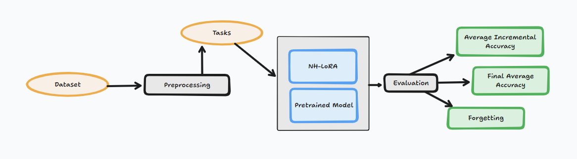
In this class incremental learning setup, the dataset is first preprocessed using PILOT to prepare the samples before they are split into a sequence of tasks. The model then learns each task step by step using a pretrained model with NH-LoRA, which helps it adapt to new classes while reducing catastrophic forgetting on previously learned ones.

After training on each incremental task, the model is evaluated using Average Incremental Accuracy, Final Average Accuracy, and Forgetting. These metrics show not only how well the model learns new classes, but also how much performance it retains on earlier classes throughout the incremental process.

Parameter config

The configuration (batch, learning-rate, etc) can be found here. It contain spesific configuration for each dataset used in this work.

Evaluation

The evaluation for our model consist of two method :

Final Average Accuracy

This metric represents the average accuracy at the very end of training, after the model has learned all tasks. In other words, it measures how well the final model performs across every task or class that has appeared so far. This is the main score used to summarize the overall final performance of the continual learning process.

It is calculated as follows:

Final Average Accuracy = \frac{1}{T} \sum_{i = 1}^{T} A_{T, i}

where:

$T$ is the total number of tasks,
$A_{T, i}$ is the accuracy on task $i$ after training the final task $T$ .

Forgetting

Forgetting measures how much performance on earlier tasks drops after the model learns new tasks. In continual learning, this is an important metric because a model may achieve high accuracy on the latest task while gradually losing knowledge from previous tasks. A lower forgetting value means the model preserves past knowledge better.

Forgetting = \frac{1}{T - 1} \sum_{i = 1}^{T - 1} (A_{i}^{b e s t} - A_{T, i})

where:

$T$ is the total number of tasks,
$A_{i}^{b e s t}$ is the best accuracy ever achieved on task $i$ before the final task,
$A_{T, i}$ is the accuracy on task $i$ after training the final task.

A higher value means more forgetting, while a lower value means better retention of previously learned tasks.

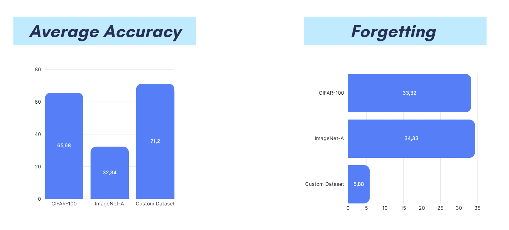
We have run 8 experiment (detailed explanation here ), and here are the best result for each dataset :

Conclusion

Well, as we can see up there, NH-LoRA does help the model learn new classes without either fully retraining from scratch or modifying all backbone parameters. The proposed adapter design is applied across all layers to preserve plasticity, which differs from methods such as CL-LoRA that rely on more specialized adapters in selected layers [2]. In this sense, the architecture is designed to adapt its structure according to task novelty and conflict, instead of using the same fixed adaptation strategy for every task. Therefore, this should improve flexibility and allow capacity to be allocated more effectively, especially when the incoming task has a different level of similarity to previous ones.

However, we still need to adjust some our expectation for the result. The model still struggles to maintain old knowledge while learning new tasks, so the forgetting issue is still present. It may benefit from the horizontal planner mechanism, yet the extra conditions and regularization also make the optimization harder if they are not well balanced.

We also have to remember that the result is also likely affected by training configuration differences, such as task split, number of epochs, learning rate, and other hyperparameters. This need to examine further, as we don't have more budget for another experiment :( , and every experiment does take time (CIFAR itself need around 5-6 hours per fine-tuning).

Future Works

For future work, NH-LoRA would benefit from more extensive experimentation, especially on parameter tuning and task-setting variations. Since continual learning performance is highly sensitive to hyperparameters, a more systematic search over learning rate, rank budget, regularization strength, and task split could give a clearer picture of the method’s true potential.

References

[1] D.-W. Zhou et al., “Class-Incremental Learning: A Survey.” 2023. [Online]. Available: https://arxiv.org/abs/2302.03648

[2] J. He, Z. Duan, and F. Zhu, “CL-LoRA: Continual Low-Rank Adaptation for Rehearsal-Free Class-Incremental Learning.” 2025. [Online]. Available: https://arxiv.org/abs/2505.24816

[3] V. Lialin et al., “Scaling Down to Scale Up: A Guide to Parameter-Efficient Fine-Tuning.” 2023. [Online]. Available: https://arxiv.org/abs/2303.15647

[4] B. Jung et al., “Neuromorphic Computing - An Overview.” 2025. [Online]. Available: https://arxiv.org/abs/2510.06721v2

[5] S. Hou et al., “Learning a Unified Classifier Incrementally via Rebalancing.” 2019. [Online]. Available: https://openaccess.thecvf.com/content_CVPR_2019/html/Hou_Learning_a_Unified_Classifier_Incrementally_via_Rebalancing_CVPR_2019_paper.html

[6] J. Yoon et al., “Lifelong Learning with Dynamically Expandable Networks.” 2018. [Online]. Available: https://openreview.net/forum?id=Bk-aoer_-

[7] A. Dosovitskiy et al., “An Image is Worth 16×16 Words: Transformers for Image Recognition at Scale.” 2020. [Online]. Available: https://arxiv.org/abs/2010.11929

[8] A. Vaswani et al., “Attention Is All You Need.” 2017. [Online]. Available: https://arxiv.org/abs/1706.03762

[9] Z. Hu et al., “Low Rank Regularization: A review.” 2021. [Online]. Available: https://www.sciencedirect.com/science/article/pii/S0893608021001468

[10] A. Rokah et al., “Mixture-of-Experts Models in Vision: Routing, Optimization, and Generalization.” 2026. [Online]. Available: https://arxiv.org/abs/2601.15021v1

[11] E. J. Hu et al., “LoRA: Low-Rank Adaptation of Large Language Models.” 2021. [Online]. Available: https://arxiv.org/abs/2106.09685

[12] Z. Li and D. Hoiem, “Learning without Forgetting.” 2016. [Online]. Available: https://arxiv.org/abs/1606.09282

Preface

Links

Problem Statement

Image Classification

(Incremental) Image Classification

Vision Transformer (ViT)

Transformer

Attention

(Vision) Transformer

Patch Embedding

Positional Encoding

NH-LoRA

Preface

PEFT (Parameter Efficient Tuning)

LoRA

Architecture

Task-State Encoder

Tasks

Warmup

Horizon Planner

Decision

Instance Router

Incremental Cosine Head

Consolidation and Homeostasis Unit

Loss Function

Training

Overview

Parameter config

Evaluation

Conclusion

Future Works

References